Overview
In this article, we will answer the questions:
- how to counteract sampling bias in LLM judges?
- how many evaluator repetitions are enough?
- how does cost scale with reliability and quality?
We will use confidence intervals to quantify the required level of score precision, and sample statistics to estimate the number of samples required to achieve that precision.
We will also derive some rules-of-thumb scaling laws for how this strategy affects the time, cost, and quality of the evaluation.
- Problem: LLM evaluators are stochastic
- Sequential Sampling Algorithm
- Mixed‑Expert Sampling
- Estimating the Number of Samples to Poll
- Scaling Laws — how each knob changes the bottom line
- Impact on Time, Cost and Quality of Evaluation
- Discussion — practical knobs & tips
We will derive that if we collect samples of a scalar evaluator's score, the expected number of samples required to achieve a % confidence interval for the mean is:
and the mean score has the following confidence interval:
where:
- is the total number of samples collected
- is the z-score for the confidence level (statistical confidence)
- is the number of bins or classes (granularity of score)
- is the range of the score (max - min)
- is the normalized sample standard deviation (noisiness/discriminative power of the evaluator)
For example, if we have the following (hidden) Likert scale with mean = 4 and std = 0.6:
Then the expected number of samples required for a 90% confidence interval for the mean is:
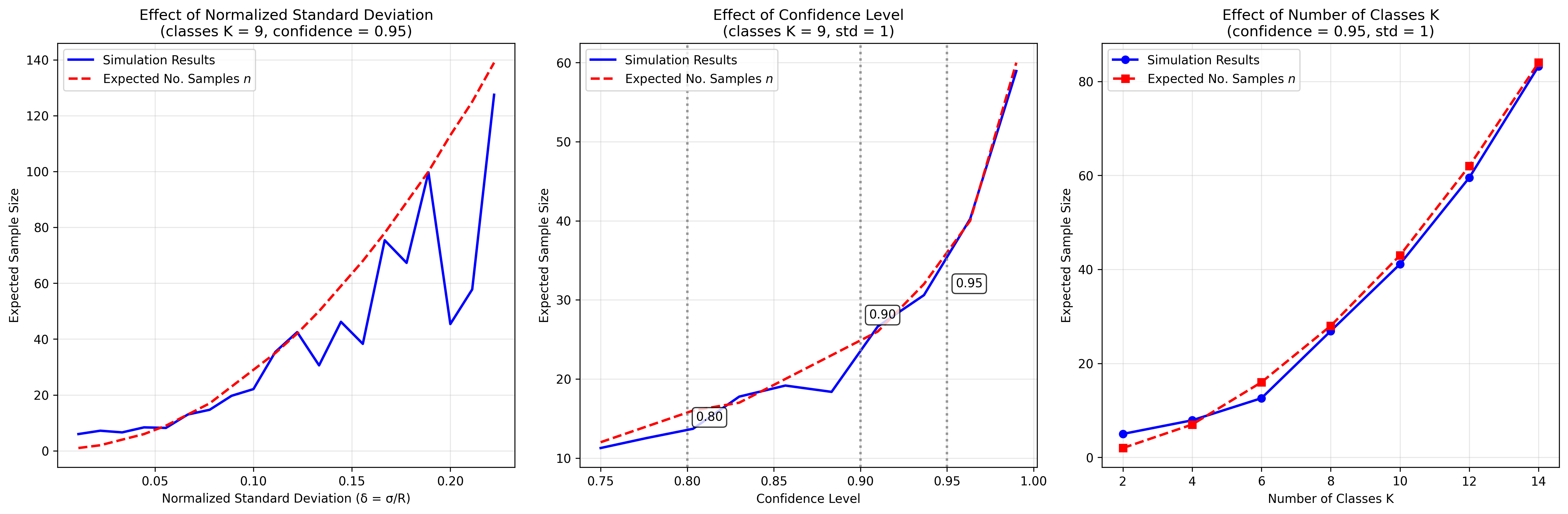
We will use simulation to see that this holds true.
Git repo with code: https://github.com/sunnybak/precision-based-sampling
Problem: LLM evaluators are stochastic
Let's say you wish to evaluate the quality of your agent's output using an LLM as a judge. You might see something as follows:
| evaluator 1 | evaluator 2 | evaluator 3 | |
|---|---|---|---|
| scores | 4 | 5 | 5 |
At face value, this might seem great. However, when you repeat the evaluators with the same prompt 5 times, the results might tell a different story
| evaluator 1 | evaluator 2 | evaluator 3 | |
|---|---|---|---|
| scores | 4, 4, 5, 5, 5 | 5, 4, 3, 4, 2 | 5, 4, 5, 4, 5 |
| mean scores | 4.6 | 3.6 | 4.6 |
| std scores | 0.55 | 1.14 | 0.55 |
Evaluator 2 seems to be producing scores that have a higher variance than the other evaluators, whereas evaluator 3 seems to be more consistent.
This does not necessarily mean that evaluator 2 is worse than evaluator 3. There are some explanations as to why evaluator 2 has more variance than evaluator 3:
- the metric measured by evaluator 2 is harder to grade, more subjective, or general
- evaluator 2 is set up to discriminate with more granularity than evaluator 3
An example of evaluator 2 could be "How well does the agent understand the user's intent?".
Evaluator 3 could be "Is the output toxic?", a metric that is easier to grade and likely has a lower variance.
Now, let's define the problem and work through the solution step by step.
Setup
Let's assume that an evaluator maps outputs to a 1D scalar score on a specific dimension (e.g., helpfulness, correctness, creativity).
This scalar score is then discretized into bins or classes — e.g., Likert 1–5 (5 classes), or binary "Pass/Fail" (2 classes).
Note: it's not recommended to evaluate on more than 1 dimension at a time, since the evaluator scores will likely be biased if multiple dimensions are evaluated at once.
Let's also assume that there is some objective truth to the score, and that the evaluator's score is a noisy estimate of that truth.
If we take samples of the evaluator's score, IID, we can estimate the mean and variance of the score.
Precision Criteria
We want to keep sampling until the two-sided confidence interval half-width is . In other words:
For example, if we want to be 95% confident that the true mean is within of the derived mean, we can set .
Now let's give more thought to the value of .
Value of the half-interval
The value of must be chosen carefully to be able to distinguish between the classes. This number depends on 2 factors:
- the range of the scale being used
- the number of bins or classes we want to sort into
The number of intervals we require are thus . The maximum half-width to ensure no overlap between the intervals is . It is best practice to also leave some buffer between the intervals so that the CI sits comfortably inside its bin, and so we use thirds instead of halves. This means that our intervals are not only disjointed, but also leave some buffer between each other, increasing precision. The formula we will use is
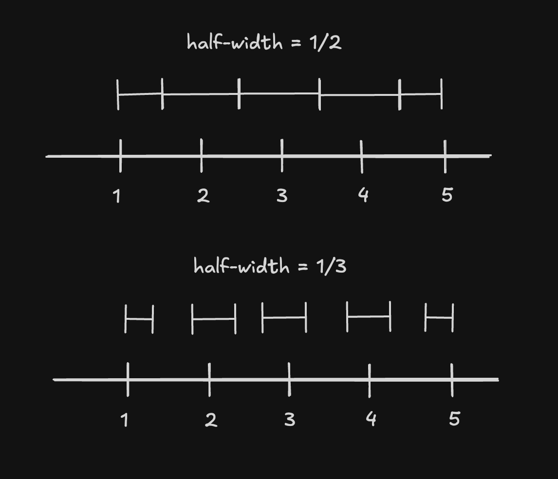
Here are some examples for different scales and their corresponding half-widths:
| Scale | Range | Classes | Half-width | Intervals |
|---|---|---|---|---|
| 1-5 | 4 | 5 | 0.267 | (0.733, 1.267), (1.733, 2.267), ... |
| 1-10 | 9 | 10 | 0.3 | (0.7, 1.3), (1.7, 2.3), ... |
| 0-1 | 1 | 3 | 0.111 | (0.899, 1.111), (1.899, 2.111), ... |
Sequential Sampling Algorithm
The sequential sampling algorithm works by iteratively collecting samples until we achieve the desired precision. Here's how it works:
- Start with a small batch of pilot samples (n0=10) to get an initial estimate of the variance
- Calculate the current confidence interval half-width (h)
- If h is small enough for the required precision (≤ d), we're done
- Otherwise, estimate how many more samples we need based on the current variance
- Collect those additional samples and repeat from step 2
The algorithm is efficient because it adapts to the variance of the data - if the evaluator is very noisy (high variance), it will collect more samples, but if the evaluator is very precise (low variance), it will collect fewer samples.
The following is a Python implementation of the sequential sampling algorithm:
async def batch_eval(n):
    # run the evaluator n times in parallel
    return run_concurrently(run_evaluator, n)

async def seq_sample(sample_batch, alpha, K, R):
    n0 = 10 # number of pilot samples
    z = st.norm.ppf(1 - alpha/2)  # z-score for the confidence interval
    x = list(await batch_eval(response, evaluator, n0))  # pilot samples
    d = R / (3 * K) # half-width of the confidence interval
    while True:
        n = len(x) # current sample size
        std = np.std(x, ddof=1) # sample standard deviation

        # Current confidence interval half-width
        h = z * std / np.sqrt(n)
        if h <= d:
            # we have enough samples
            break

		delta = std / R # normalized sample standard deviation
        n_req = math.ceil((3 * z * K * delta) ** 2) # total number of samples required
        # Get more samples, but limit batch size
        n_additional = max(1, min(n_req - n, n0))
        additional_samples = await batch_eval(response, evaluator, n_additional)
        x.extend(additional_samples)
    return np.mean(x) # return the mean of the samples
You can find the full implementation in the repo: https://github.com/sunnybak/precision-based-sampling.
Mixed‑Expert Sampling
Given that we assume some true mean which is (theoretically) model-agnostic, one way to improve robustness is to sample from multiple LLMs as judges in the same batch and treat each judge's vote as another IID sample. This will lead to robustness while requiring no change to the algorithm or scaling laws. Here's how we can implement this in Python:
- make a list of LLM models to sample from and set up their keys
- use konfigure for managing prompts and parameters
- use Python
cycleto cycle through the models in a round-robin fashion (also add asyncio/thread locking) - use litellm for model routing
- sample from each model in the list using the cycle
Here's a simple implementation of mixed-expert sampling:
import konfigure
from litellm import acompletion

config = konfigure.load('/path/to/config.yaml')

model_cycle = cycle(config.models)
prompt_cycle = cycle(config.prompts)
cycle_lock = asyncio.Lock()

async def get_llm_rating(response: str) -> Optional[int]:
    rating = None
    try:
        # Get next model in a thread-safe way
        async with cycle_lock:
            selected_model = next(model_cycle)
            selected_prompt = next(prompt_cycle)

        response = await acompletion(
            model=selected_model,
            messages=[{
                "role": "user",
                "content": selected_prompt.render(
                    response=response,
                    likert_scale_min=LIKERT_SCALE_MIN,
                    likert_scale_max=LIKERT_SCALE_MAX,
                )
            }],
        )
        content = response.choices[0].message.content
        rating = int(content)
    except Exception as e:
        return None

    return rating
The full implementation is in the repo: https://github.com/sunnybak/precision-based-sampling.
Estimating the Number of Samples to Poll
- CI width (large‑ normal approximation)
- Precision target from the one‑third‑gap rule
- Solve for
Since we don't know the true standard deviation , we can replace it by the sample standard deviation to get the estimated number of samples required to achieve the desired precision:
Let us define the normalized scale-invariant sample standard deviation as
This is because we want to know the amount of variation irrespective of the scale being used. Finally, we get:
Scaling Laws — how each knob changes the bottom line
Expected Number of Samples
The expected number of total samples needed to achieve a % confidence interval, , is:
where
- is the z-score for the confidence level (statistical confidence)
- is the number of bins or classes (granularity of score)
- is the normalized sample standard deviation (noisiness/discriminative power of the evaluator)
Based on this, we get the following relationships:
- Confidence level : Sharper CIs get expensive slowly (log‑like). 95% → 99% multiplies by only ≈ 1.7. Reliability is relatively inexpensive!
- Normalized Std‑dev : Halving variability quarters the required runs. If the evaluator has more variability, quadratically more samples are needed to be confident. This value is high for evaluators which produce a wider range of scores.
- Number of Bins : Increasing the number of bins for the same range will quadratically increase the number of samples required, because we want higher granularity. For example, if a 0-1 scale with 2 bins will require 6 samples, but a 0-1 scale with 4 bins will require 36 samples.
Impacts on Time, Cost and Quality of Evaluation
- Since the number of input and output tokens are the same, cost is directly proportional to the total number of samples, assuming constant price per token.
- The latency is proportional to the number of concurrent calls made to the LLM, which is . Increasing the minimum and maximum batch sizes will cause a faster convergence, but can lead to overshooting the number of samples required.
- Quality is some function of the confidence level and the half-width . Lower values of and will improve the reliability and granularity of the metric.
Discussion — practical knobs & tips
Initial sample size
A pilot of 5-10 samples gives a tolerant first variance estimate. If you have historical data, use its to seed before the first run.
Batch size
If the batch size is too large, the latency will increase - there are always some API calls that take much longer. From experiments, I have found that 5-10 concurrent API calls work best for OpenAI.
Here's a latency plot for concurrent API calls for GPT-4.1
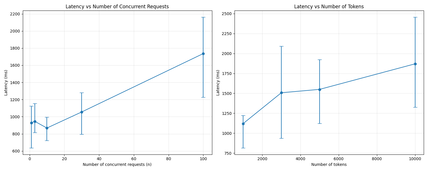
As you can see, the error bars in the latency increase with the number of concurrent API calls, pushing the mean latency up.
What if is still huge?
Depending on your use case, you might want to tune the cost, latency, or quality by adjusting :
- Tighten the evaluator rubric so drops. A more specific rubric which activates infrequently will have a lower .
- Accept 90% CIs instead of 95%.
- Reduce classes: 1-10 ratings -> 1-5 ratings will reduce by half and the cost by a quarter.
Git repo with code: https://github.com/sunnybak/precision-based-sampling